Jun 11, 2020 by Yassine long-read deep-learning semi-supervised

[A more detailed version of this post is available on arXiv.]
[A curated and an up-to-date list of SSL papers is available on github.]

Deep neural networks demonstrated their ability to provide remarkable performances on certain supervised learning tasks (e.g., image classification) when trained on extensive collections of labeled data (e.g. ImageNet). However, creating such large collections of data requires a considerable amount of resources, time, and effort. Such resources may not be available in many practical cases, limiting the adoption and application of many deep learning (DL) methods.

In a search for more data-efficient DL methods to overcome the need for large annotated datasets, we see a lot of research interest in recent years with regards to the application of semi-supervised learning (SSL) to deep neural nets as a possible alternative, by developing novel methods and adopting existing SSL frameworks for a deep learning setting. This post discusses SSL in a deep learning setting and goes through some of the main deep learning SSL methods.

Semi-supervised Learning
Consistency Regularization
Entropy Minimization
Proxy-label Methods
Holistic Methods
References

Semi-supervised Learning

What is Semi-supervised Learning?

Semi-supervised learning (SSL) is halfway between supervised and unsupervised learning. In addition to unlabeled data, the algorithm is provided with some supervision information – but not necessarily for all examples. Often, this information will be the targets associated with some of the examples. In this case, the data set \( X=\left(x_{i}\right); i \in [n]\) can be divided into two parts: the points \( X_{l}:=\left(x_{1}, \dots, x_{l}\right) \), for which labels \( Y_{l}:=\left(y_{1}, \dots, y_{l}\right) \) are provided, and the points \( X_{u}:=\left(x_{l+1}, \ldots, x_{l+u}\right) \), the labels of which are not known.

Chapelle et al. — SSL book

As stated in the definition above, in SSL, we are provided with a dataset containing both labeled and unlabeled examples. The portion of labeled examples is usually quite small compared to the unlabeled example (e.g., 1 to 10% of the total number of examples). So with a dataset \(\mathcal{D}\) containing a labeled subset \(\mathcal{D}_l\) and an unlabeled subset \(\mathcal{D}_u\). The objective, or rather hope, is to leverage the unlabeled examples to train a better performing model than what can be obtained using only the labeled portion. And hopefully, get closer to the desired optimal performance, in which all of the dataset \(\mathcal{D}\) is labeled.

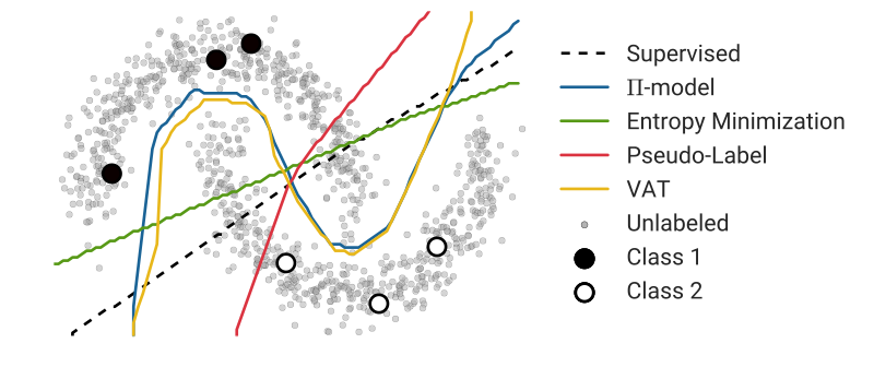
More formally, SSL’s goal is to leverage the unlabeled data \(\mathcal{D}_u\) to produce a prediction function \(f_{\theta}\) with trainable parameters \(\theta\), that is more accurate than what would have been obtained by only using the labeled data \(\mathcal{D}_l\). For instance, \(\mathcal{D}_u\) might provide us with additional information about the structure of the data distribution \(p(x)\), to better estimate the decision boundary between the different classes. As shown in Fig. 1 bellow, where the data points with distinct labels are separated with low-density regions, leveraging unlabeled data with a SSL approach can provide us with additional information about the shape of the decision boundary between two classes and reduce the ambiguity present in the supervised case.

Fig. 1. The decision boundaries obtained on two moons dataset, with a supervised and different SSL approaches, using 6 labeled examples, 3 for each class and the rest of the points as unlabeled data. (Image source: Oliver et al)

Semi-supervised learning first appeared in the form of self-training, where a model is first trained on labeled data, and then, iteratively, at each training iteration, a portion of the unlabeled data is annotated using the trained model and added to the training set for the next iteration. SSL really took off in the 1970s after its success with iterative algorithms such as the expectation-maximization algorithm, using labeled and unlabeled data to maximize the likelihood of the model. In this post, we are only interested in SSL applied to deep learning. For a detailed review of the field, Semi-Supervised Learning Book is a good resource.

Semi-supervised learning methods

There have been many SSL methods and approaches that have been introduced over the years, SSL algorithms can be broadly divided into the following categories:

Consistency Regularization (Consistency Training). Based on the assumption that if a realistic perturbation was applied to the unlabeled data points, the prediction should not change significantly. We can then train the model to have a consistent prediction on a given unlabeled example and its perturbed version.
Proxy-label Methods. Such methods leverage a trained model on the labeled set to produce additional training examples extracted from the unlabeled set based on some heuristic. These approaches can also be referred to as self-teaching or bootstrapping algorithms; we follow Ruder et al. and refer to them as proxy-label methods. Some examples of such methods are Self-training, Co-training, and Multi-View Learning.
Generative models. Similar to the supervised setting, where the learned features on one task can be transferred to other downstream tasks. Generative models that are able to generate images from the data distribution \(p(x)\) must learn transferable features to a supervised task \(p(x | y)\) for a given task with targets \(y\).
Graph-Based Methods. A labeled and unlabeled data points constitute the nodes of the graph, and the objective is to propagate the labels from the labeled nodes to the unlabeled ones. The similarity of two nodes \(n_i\) and \(n_j\) is reflected by how strong is the edge \(e_{ij}\) between them.

In addition to these main categories, there is also some SSL work on entropy minimization, where we force the model to make confident predictions by minimizing the entropy of the predictions. Consistency training can also be considered as a proxy-label method, with a subtle difference where instead of considering the predictions as ground-truths and compute the cross-entropy loss, we enforce consistency of predictions by minimizing a given distance between the outputs.

In this post, we will focus more on consistency regularization based approaches, given that they are the most commonly used methods in deep learning, and we will present a brief introduction to the proxy-label, and holistic approaches.

Main Assumptions in SSL

The first question we need to answer, is under what assumptions can we apply SSL algorithms? SSL algorithms only work under some conditions, where some assumptions about the structure of the data need to hold. Without such assumptions, it would not be possible to generalize from a finite training set to a set of possibly infinitely many unseen test cases.

The main assumptions in SSL are:

The Smoothness Assumption: If two points \(x_1\), \(x_2\) that reside in a high-density regions are close, then so should be their corresponding outputs \(y_1\), \(y_2\). Meaning that if two inputs are of the same class and belong to the same cluster, which is a high-density region of the input space, then their corresponding outputs need to be close. The inverse holds; if the two points are separated by a low-density region, the outputs must be distant from each other. This assumption can be quite helpful in a classification task, but not so much for regression.
The Cluster Assumption: If points are in the same cluster, they are likely to be of the same class. In this special case of the smoothness assumption, we suppose that input data points form clusters, and each cluster corresponds to one of the output classes. The cluster assumption can also be seen as the low-density separation assumption: the decision boundary should lie in the low-density regions. The relation between the two assumptions is easy to see, if a given decision boundary lies in a high-density region, it will likely cut a cluster into two different classes, resulting in samples from different classes belonging to the same cluster, which is a violation of the cluster assumption. In this case, we can restrict our model to have consistent predictions on the unlabeled data over some small perturbations pushing its decision boundary to low-density regions.
The Manifold Assumption: The (high-dimensional) data lie (roughly) on a low-dimensional manifold. With high dimensional space, where the volume grows exponentially with the number of dimensions, it can be quite hard to estimate the true data distribution for generative tasks, and for discriminative tasks, the distances are similar regardless of the class type, making classification quite challenging. However, if our input data lies on some lower-dimensional manifold, we can try to find a low dimensional representation using the unlabeled data and then use the labeled data to solve the simplified task.

Consistency Regularization

A recent line of works in deep semi-supervised learning utilize the unlabeled data to enforce the trained model to be in line with the cluster assumption, i.e., the learned decision boundary must lie in low-density regions. These methods are based on a simple concept that, if a realistic perturbation was to be applied to an unlabeled example, the prediction should not change significantly, given that under the cluster assumption: Data points with distinct labels are separated with low-density regions, so the likelihood of one example switching classes after a perturbation is small (see Figure 1).

More formally, with consistency regularization, we are favoring the functions \(f_\theta\) that give consistent prediction for similar data points. So rather than minimizing the classification cost at the zero-dimensional data points of the inputs space, the regularized model minimizes the cost on a manifold around each data point, pushing the decision boundaries away from the unlabeled data points and smoothing the manifold on which the data resides (Zhu, 2005). Given an unlabeled data point \(x_u \in \mathcal{D}_u\) and its perturbed version \(\hat{x}_u\), the objective is to minimize the distance between the two outputs \(d(f_{\theta}(x_u), f_{\theta}(\hat{x}_u))\). The popular distance measures \(d\) are mean squared error (MSE), Kullback-Leiber divergence (KL) and Jensen-Shannon divergence (JS). For two outputs \(y_u = f_{\theta}(x_u)\) and \(\hat{y}_u = f_{\theta}(\hat{x}_u)\) in the form of a probability distribution over the \(C\) classes, and \(m=\frac{1}{2}(f_{\theta}(x_u) + f_{\theta}(\hat{x}_u))\), we can compute these measures as follows:

\[\small d_{\mathrm{MSE}}(y_u, \hat{y}_u)=\frac{1}{C} \sum_{k=1}^{C}(f_{\theta}(x_u)_k -f_{\theta}(\hat{x}_u)_k)^{2}\] \[\small d_{\mathrm{KL}}(y_u, \hat{y}_u)=\frac{1}{C} \sum_{k=1}^{C} f_{\theta}(x_u)_k \log \frac{f_{\theta}(x_u)_k}{f_{\theta}(\hat{x}_u)_k}\] \[\small d_{\mathrm{JS}}(y_u, \hat{y}_u)=\frac{1}{2} d_{\mathrm{KL}}(y_u, m)+\frac{1}{2} \mathrm{d}_{\mathrm{KL}}(\hat{y}_u, m)\]

Note that we can also enforce a consistency over two perturbed versions of \(x_u\), \(\hat{x}_{u_1}\) and \(\hat{x}_{u_2}\). Now let’s go through the popular consistency regularization methods in deep learning.

Ladder Networks

With the objective to take any well-performing feed-forward network on supervised data and augment it with additional branches to be able to utilize additional unlabeled data. Rasmus et al. proposed to use Ladder Networks (Harri Valpola) with an additional encoder and decoder for SSL. As illustrated in Figure 2, the network consists of two encoders, a corrupted and clean one, and a decoder. At each training iteration, the input \(x\) is passed through both encoders. In the corrupted encoder, Gaussian noise is injected at each layer after batch normalization, producing two outputs, a clean prediction \(y\) and a prediction based on corrupted activations \(\tilde{y}\). The output \(\tilde{y}\) is then fed into the decoder to reconstruct the uncorrupted input and the clean hidden activations. The unsupervised training loss \(\mathcal{L}_u\) is then computed as the MSE between the activations of the clean encoder \(\mathbf{z}\) and the reconstructed activations \(\hat{\mathbf{z}}\) (ie., after batch normalization) in the decoder using the corrupted output \(\tilde{y}\), this is computed over all layers, from the input to the last layer \(L\), with a weighting \(\lambda_{l}\) for each layer’s contribution loss:

\[\mathcal{L}_u = \frac{1}{|\mathcal{D}|} \sum_{x \in \mathcal{D}} \sum_{l=0}^{L} \lambda_{l}\|\mathbf{z}^{(l)}-\hat{\mathbf{z}}^{(l)}\|^{2}\]

If the input \(x\) is a labeled data point (\(x \in \mathcal{D}_l\)). Then we can add a supervised loss term to \(\mathcal{L}_u\) to obtain the final loss. Note the supervised cross-entropy \(\mathrm{H}(\tilde{y}, t)\) loss is computed between the corrupted output \(\tilde{y}\) and the targets \(t\):

\[\mathcal{L} = \mathcal{L}_u + \mathcal{L}_s = \mathcal{L}_u + \frac{1}{|\mathcal{D}_l|} \sum_{x, t \in \mathcal{D}_l} \mathrm{H}(\tilde{y}, t)\]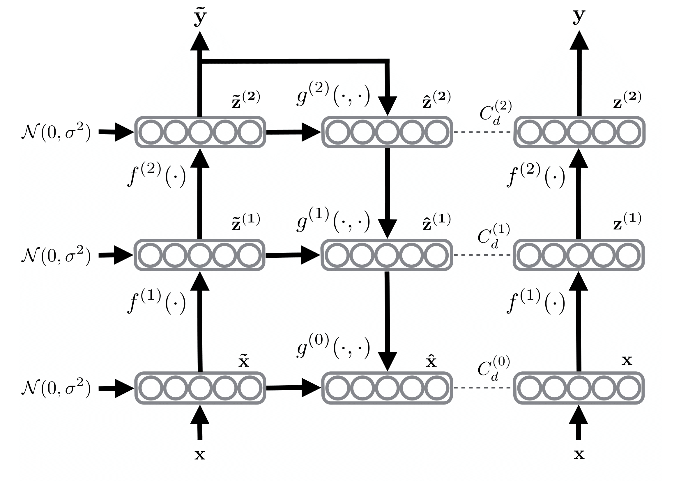

Fig. 2. An illustration of one forward pass of Ladder Networks, C refers to the MSE loss between the activations at various layers. (Image source: Rasmus et al)

The method can be easily adapted for convolutional neural networks (CNNs) by replacing the fully-connected layers with convolution and deconvolution layers for semi-supervised vision tasks. However, the ladder network is quite heavy computationally, approximately tripling the computation needed for one training iteration. To mitigate this, the authors propose a variant of ladder networks called Γ-Model where \(\lambda_{l}=0\) when \(l<L\). In this case, the decoder is omitted, and the unsupervised loss is computed as the MSE between the two outputs \(y\) and \(\tilde{y}\).

Π-model

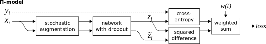
The Π-model (Laine et al.) is a simplification of the Γ-Model of Ladder Networks, where the corrupted encoder is removed, and the same network is used to get the prediction for both corrupted and uncorrupted inputs. Specifically, Π-model takes advantage of the stochastic nature of the prediction function \(f_ \theta\) in neural networks due to conventional regularization techniques, such as data augmentation and dropout, that typically don’t alter the model’s predictions. For any given input \(x\), the objective is to reduce the distances between two predictions of \(f_ \theta\) with \(x\) as input in both forward passes. Concretely, as illustrated in Figure 3, we would like to minimize \(d(z, \tilde{z})\), where we consider one of the two outputs as a target. Given the stochastic nature of the predictions function (ie., using dropout as noise source), the two outputs \(f_\theta(x) = z\) and \(f_\theta(x) = \tilde{z}\) will be distinct. The objective is to obtain consistent predictions for both of them. In case the input \(x\) is a labeled data point, we also compute the cross-entropy supervised loss using the provided labels \(y\) and the total loss will be:

\[\mathcal{L} = w \frac{1}{|\mathcal{D}_u|} \sum_{x \in \mathcal{D}_u} d_{\mathrm{MSE}}(z, \tilde{z}) + \frac{1}{|\mathcal{D}_l|} \sum_{x, y \in \mathcal{D}_l} \mathrm{H}(y, z)\]

With \(w\) as a weighting function, starting from 0 up to a fixed weight \(\lambda\) (eg., 30) after a given number of epochs (eg., 20% of training time). This way, we avoid using the untrained and random prediction function providing us with unstable predictions at the start of training to extract the training signal from the unlabeled examples.

Fig. 3. Loss computation for **Π-model**, we compute the MSE between the two outputs for the unsupervised loss, and if the input is a labeled example, we add the supervised loss to the weighted unsupervised loss. (Image source: Laine et al)

Temporal Ensembling

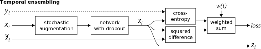
Π-model can be divided into two stages. We first classify all of the training data without updating the weights of the model, obtaining the predictions \(\tilde{z}\), and in the second stage, we consider the predictions \(\tilde{z}\) as targets for the unsupervised loss and enforce consistency of predictions by minimizing the distance between the current outputs \(z\) and the outputs of the first stage \(\tilde{z}\) under different dropout and augmentations. The problem with this approach is that the targets \(\tilde{z}\) are based on a single evaluation of the network and can rapidly change, this instability in the targets can lead to instability during training and reduces the amount of training signal that can be extracted from the unlabeled examples. To solve this, Laine et al. proposed a second version of Π-model called Temporal Ensembling, where the targets \(\tilde{z}\) are the aggregation of all the previous predictions. This way, during training, we only need a single forward pass to get the current predictions \(z\) and the aggregated targets \(\tilde{z}\), speeding up the training time by approximately 2x. The training process is illustrated in Figure 4.

For a target \(\tilde{z}\), at each training iteration, the current output \(z\) are accumulated into the ensemble outputs \(\tilde{z}\) by an exponentially moving average update:

\[\tilde{z} = \alpha \tilde{z}+(1-\alpha) z\]

where \(\alpha\) is a momentum term that controls how far the ensemble reaches into training history. \(\tilde{z}\) can also be seen as the output of an ensemble network \(f\) from previous training epochs, where the recent ones have a greater weight than the distant ones.

At the start of training, temporal ensembling reduces to Π-model since the aggregated targets are very noisy, to overcome this, similar to the bias correction used in Adam optimizer, a training target \(\tilde{z}\) are corrected for the startup bias at a training step \(t\) as follows:

\[\tilde{z} = (\alpha \tilde{z}+(1-\alpha) z) / (1-\alpha^{t})\]

The loss computation in temporal ensembling remains the same as in Π-model, but with two critical benefits. First, the training is faster since we only need a single forward pass through the network to obtain \(z\), while maintaining an exponential moving average (EMA) of label predictions on each training example, and penalizes predictions that are inconsistent with these targets. Second, the targets are more stable during training, yielding better results. The downside of such a method is a large amount of memory needed to keep an aggregate of the predictions for all of the training examples, which can become quite memory intensive for large datasets and dense tasks (e.g., semantic segmentation).

Mean Teachers

In the previous approach, the same model plays a dual role as a teacher and a student. Given a set of unlabeled data, as a teacher, the model generates the targets, which are then used by itself as a student for learning using a consistency loss. These targets may very well be misclassified, and if the weight of the unsupervised loss outweighs that of the supervised loss, the model is prevented from learning new information and keeps predicting the same targets, resulting in the form of confirmation bias. To solve this, the quality of the targets must be improved.

The quality of targets can be improved by either: (1) carefully choosing the perturbations instead of simply injecting additive or multiplicative noise, or (2) carefully choosing the teacher model responsible for generating the targets, instead of using a replica of the student model.

Π-model and its improved version with Temporal Ensembling provides a better and more stable teacher model by maintaining an EMA of the predictions of each example, which is formed by an ensemble of the model’s current version and those earlier versions that evaluated the same example. This ensembling improves the quality of the predictions and using them as the teacher predictions improve results. However, the newly learned information is incorporated into the training at a slow pace, since each target is updated only once during training, and the larger the dataset, the bigger the span between the updates gets. To overcome the limitations of Temporal Ensembling, Tarvainen et al. propose to average the model weights instead of its predictions and call this method Mean Teacher, illustrated in Figure 5.

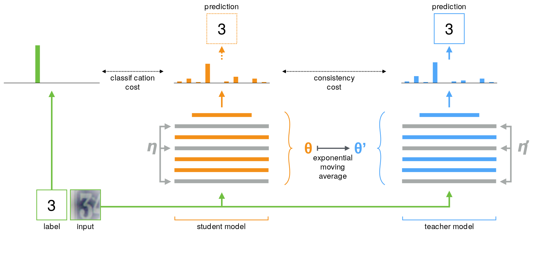
Fig. 5. The Mean Teacher method. The teacher model, which is an EMA of the student model, is responsible for generating the targets for consistency training. The student model is then trained to minimize the supervised loss over labeled examples and the consistency loss over unlabeled examples. At each training iteration, both models are evaluated with an injected noise (η, η'), and the weights of the teacher model are updated using the current student model to incorporate the learned information at a faster pace. (Image source: Tarvainen et al.)

A training iteration of Mean Teacher is very similar to previous methods. The main difference is that were the Π-model uses the same model as a student and a teacher \(\theta^{\prime}=\theta\), and temporal ensembling approximate a stable teacher \(f_{\theta^{\prime}}\) as an ensemble function with a weighted average of successive predictions. Mean Teacher defines the weights \(\theta^{\prime}_t\) of the teacher model \(f_{\theta^{\prime}}\) at training step \(t\) as the EMA of successive student’s weights \(\theta\) as follows:

\[\theta_{t}^{\prime}=\alpha \theta_{t-1}^{\prime}+(1-\alpha) \theta_{t}\]

In this case, the loss computation is the sum of the supervised and unsupervised loss, where the teacher model is used to obtain the targets for the unsupervised loss for a given input \(x_i\):

\[\mathcal{L} = w \frac{1}{|\mathcal{D}_u|} \sum_{x \in \mathcal{D}_u} d_{\mathrm{MSE}}(f_{\theta}(x), f_{\theta^{\prime}}(x)) + \frac{1}{|\mathcal{D}_l|} \sum_{x, y \in \mathcal{D}_l} \mathrm{H}(y, f_{\theta}(x))\]

Dual Students

One of the main drawbacks of using Mean Teacher, where the teacher’s weights are an EMA of the student’s weights, is that given a large number of training iterations, the weights of the teacher model will converge to that of the student model, and any biased and unstable predictions will be carried over to the student.

To solve this, Ke et al. propose a dual students step-up, where two student models with different initialization are simultaneously trained, and at a given iteration, one of them provides the targets for the other. To choose which one, we check for the most stable predictions that satisfy the following stability conditions:

The predictions using two input versions, a clean \(x\) and a perturbed version \(\tilde{x}\) give the same results: \(f(x) = f(\tilde{x})\).
Both predictions are confident, ie, are far from the decision boundary. This can be tested by seeing if \(f(x)\) (resp. \(f(\tilde{x})\)) is greater than a confidence threshold \(\epsilon\), such as 0.1.

Given two student models, \(f_{\theta_1}\) and \(f_{\theta_2}\), an unlabeled input \(x_u\) and its perturbed version \(\tilde{x}_u\). We compute four predictions: \(f_{\theta_1}(x_u), f_{\theta_1}(\tilde{x}_u), f_{\theta_2}(x_u), f_{\theta_2}(\tilde{x}_u)\). In addition to training each model to minimize both the supervised and unsupervised losses for both models:

\[\mathcal{L}_s = \frac{1}{|\mathcal{D}_l|} \sum_{x_l, y \in \mathcal{D}_l} \mathrm{H}(y, f_{\theta_i}(x_l))\] \[\mathcal{L}_u = \frac{1}{|\mathcal{D}_u|} \sum_{x_u \in \mathcal{D}_u} d_{\mathrm{MSE}}(f_{\theta_i}(x_u), f_{\theta_i}(\tilde{x}_u))\]

We also force one of the students to have a similar prediction to its counterpart. To chose which one to update its weights, we check for the stability constraint for both models. If the predictions one of the models is unstable, we update its weights. If both are stable, we update the model with the largest variation \(\mathcal{E}^{i} =\left\|f_{i}(x_u)-f_{i}(\tilde{x}_u)\right\|^{2}\), so the least stable.

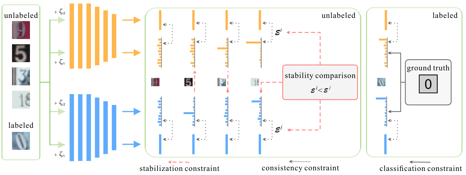
Fig. 6. Examples of the perturbed inputs for different values of the scaling hyperparameter Ɛ. (Image source: Ke et al)

In the end, as depicted in Figure 6, the least stable model is trained with the following loss:

\[\mathcal{L} = \mathcal{L}_s + \lambda_{1} \mathcal{L}_u + \lambda_{2} \frac{1}{|\mathcal{D}_u|} \sum_{x_u \in \mathcal{D}_u} d_{\mathrm{MSE}}(f_{\theta_i}(x_u), f_{\theta_j}(x_u))\]

while the stable model is trained using traditional loss for consistency training: \(\lambda_{1} \mathcal{L}_u + \mathcal{L}_s\).

Virtual Adversarial Training

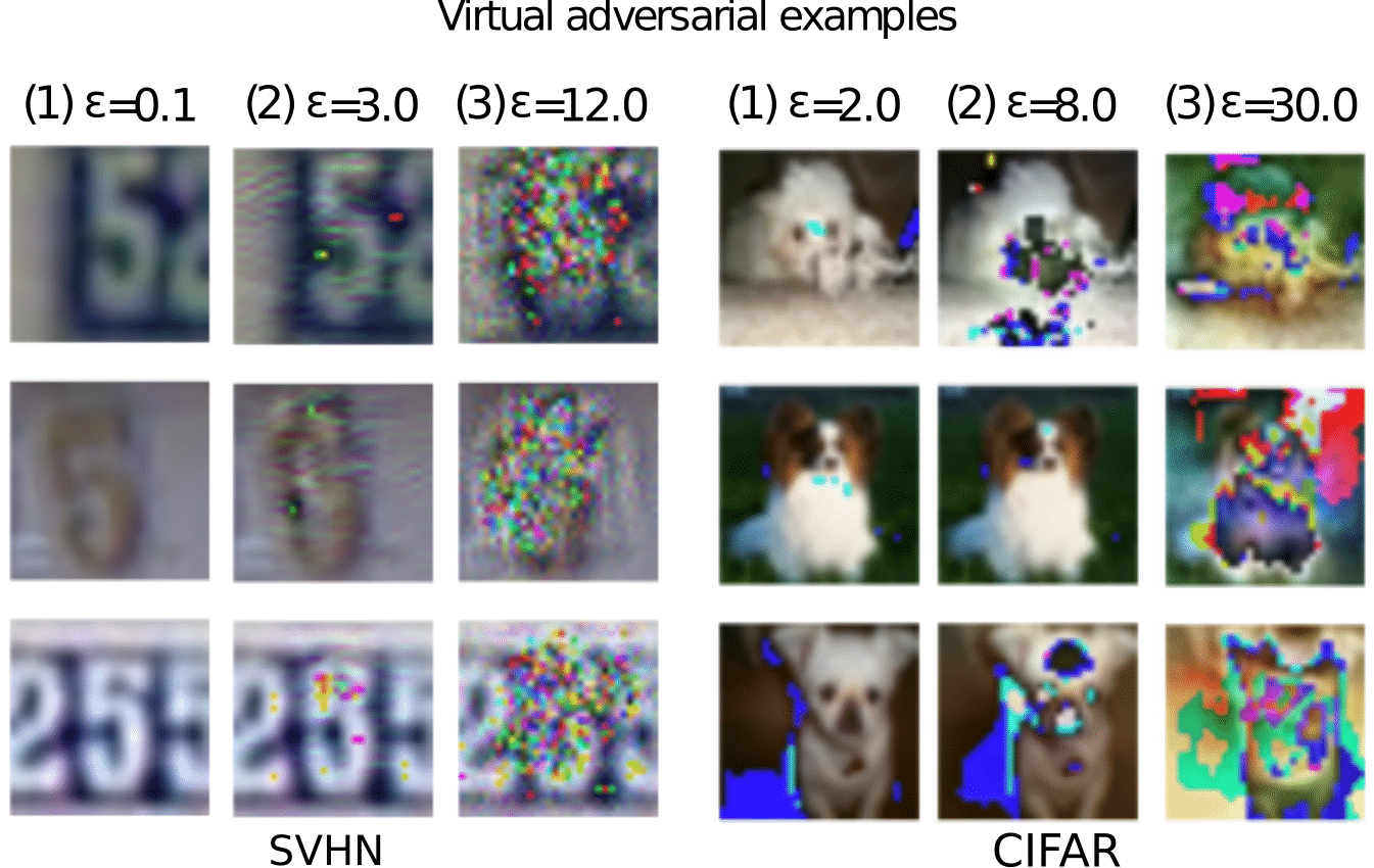
The previous approaches focused on applying random perturbations to each input to generate artificial input points, encouraging the model to assign similar outputs to the unlabeled data points and their perturbed versions, this way we push for a smoother output distribution, and as a result, the generalization performance of the model can be improved. Such random noise and random data augmentation often leaves the predictor particularly vulnerable to small perturbations in a specific direction, that is, the adversarial direction, which is the direction in the input space in which the label probability \(p(y|x)\) of the model is most sensitive.

To solve this, and inspired by adversarial training (Goodfellow et al.) that trains the model to assign to each input data a label that is similar to the labels to be assigned to its neighbors in the adversarial direction. Miyato et al. propose Virtual Adversarial Training (VAT), a regularization technique that enhances the model’s robustness around each input data point against random and local perturbations. The term “virtual” comes from the fact that the adversarial perturbation is approximated without label information and is hence applicable to semi-supervised learning to smooth the output distribution.

Concretely, VAT trains the output distribution to be identically smooth around each data point by selectively smoothing the model in its most adversarial direction. For a given data point \(x\), we would like to compute the adversarial perturbation \(r_{adv}\) that will alter the model’s predictions the most. We start by sampling a Gaussian noise \(r\) of the same dimensions as the input \(x\). We then compute its gradients \(grad_r\) with respect the loss between the two predictions, with and without the injections of the noise \(r\) (i.e., KL-divergence is used as a distance measure \(d(.,.)\)). \(r_{adv}\) can then be obtained by normalizing and scaling \(grad_r\) by a hyperparameter \(\epsilon\). This can be written as follows:

\[1) \ \ r \sim \mathcal{N}(0, \frac{\xi}{\sqrt{\operatorname{dim}(x)}} I)\] \[2) \ \ grad_{r}=\nabla_{r} d_{\mathrm{KL}}(f_{\theta}(x), f_{\theta}(x+r))\] \[3) \ \ r_{adv}=\epsilon \frac{grad_{r}}{\|grad_{r}\|}\]

Note that the computation above is a single iteration of the approximation of \(r_{adv}\), for a more accurate approximation, we consider \(r_{adv} = r\) and recompute \(r_{adv}\) following the last two steps. But in general, given how computationally expensive this computation is, requiring additional forward and backward passes, we only apply a single power iteration for computing the adversarial perturbation.

With the optimal perturbation \(r_{adv}\), we can then compute the unsupervised loss as the MSE between the two predictions of the model, with and without the injection of \(r_{adv}\):

\[\mathcal{L}_u = w \frac{1}{|\mathcal{D}_u|} \sum_{x_u \in \mathcal{D}_u} d_{\mathrm{MSE}}(f_{\theta}(x_u), f_{\theta}(x_u + r_{adv}))\]

For a more stable training, we can use a mean teacher to generate stable targets by replacing \(f_{\theta}(x_u)\) with \(f_{\theta^{\prime}}(x_u)\), where \(f_{\theta^{\prime}}\) is an EMA teacher model of the student \(f_{\theta}\).

Fig. 7. Examples of the perturbed inputs for different values of the scaling hyperparameter Ɛ. (Image source: Miyato et al)

Adversarial Dropout

Instead of using an additive adversarial noise as VAT, Park et al. propose adversarial dropout (AdD), in which dropout masks are adversarially optimized to alter the model’s predictions. With this type of perturbations, we induce a sparse structure of the neural network, while the other forms of additive noise do not make changes to the structure of the neural network directly.

The first step is to find the dropout conditions that is most sensitive to the model’s predictions. In a SSL setting, where we do not have access to the true labels, we use the model predictions on the unlabeled data points to approximate the adversarial dropout mast \(\epsilon^{adv}\), which is subject to the boundary condition: \(\|\epsilon^{adv}-\epsilon\|_{2} \leq \delta H\) with \(H\) as the dropout layer dimension and a hyperparameter \(\delta\), which restricts adversarial dropout mask to be infinitesimally different from the random dropout mask \(\epsilon\). Without this constraint, the adversarial dropout might induce a layer without any connections. By restricting the adversarial dropout to be similar to the random dropout, we prevent finding such an irrational layer, which does not support backpropagation.

Similar to VAT, we start from a random dropout mask, we compute a KL-divergence loss between the outputs with and without dropout, and given the gradients of the loss with respect to the activations before the dropout layer, we update the random dropout mask in an adversarial manner. The prediction function \(f_{\theta}\) is divided into two parts, \(f_{\theta_1}\) and \(f_{\theta_2}\), where \(f_{\theta}(x_i, \epsilon)=f_{\theta_{2}}(f_{\theta_{1}}(x_i) \odot \epsilon)\), we start by computing an approximation of the jacobian matrix as follows:

\[J(x_i, \epsilon) \approx f_{\theta_{1}}(x_i)\odot \nabla_{f_{\theta_{1}}(x_i)} d_{\mathrm{KL}}(f_{\theta}(x_i), f_{\theta}(x_i, \epsilon))\]

Using \(J(x_i, \epsilon)\), we can then update the random dropout mask \(\epsilon\) to obtain \(\epsilon^{adv}\), so that if \(\epsilon(i) = 0\) and \(J(x_i, \epsilon)(i) > 0\) or \(\epsilon(i) = 1\) and \(J(x_i, \epsilon)(i) < 0\) at a given position \(i\), we inverse the value of \(\epsilon\) at that location. Resulting in \(\epsilon^{adv}\), which can then be used to compute the unsupervised loss:

\[\mathcal{L}_u = w \frac{1}{|\mathcal{D}_u|} \sum_{x_u \in \mathcal{D}_u} d_{\mathrm{MSE}}(f_{\theta}(x_u), f_{\theta}(x_u, \epsilon^{adv}))\]

Interpolation Consistency Training

As discussed earlier, the random perturbations are inefficient in high dimensions, given that only a limited subset of the input perturbations are capable of pushing the decision boundary into low-density regions. VAT and AdD find the adversarial perturbations that will maximize the change in the model’s predictions, which involve multiple forward and backward passes to compute these perturbations. This additional computation can be restrictive in many cases and makes such methods less appealing. As an alternative, Verma et al. propose Interpolation Consistency Training (ICT) as an efficient consistency regularization technique for SSL.

Given a mixup operation \(\operatorname{Mix}_{\lambda}(a, b)=\lambda \cdot a+(1-\lambda) \cdot b\) that outputs an interpolation between the two inputs with a weight \(\lambda \sim \operatorname{Beta}(\alpha, \alpha)\) for \(\alpha \in(0, \infty)\). As shown in Figure 8, ICT trains a prediction function \(f_{\theta}\) to provide consistent predictions at different interpolations of unlabeled data points \(u_i\) and \(u_j\), where the targets are generated using a teacher model \(f_{\theta^{\prime}}\) which is an EMA of \(f_{\theta}\):

\[f_{\theta}(\operatorname{Mix}_{\lambda}(u_{j}, u_{k})) \approx \operatorname{Mix}_{\lambda}(f_{\theta^{\prime}}(u_{j}), f_{\theta^{\prime}}(u_{k}))\]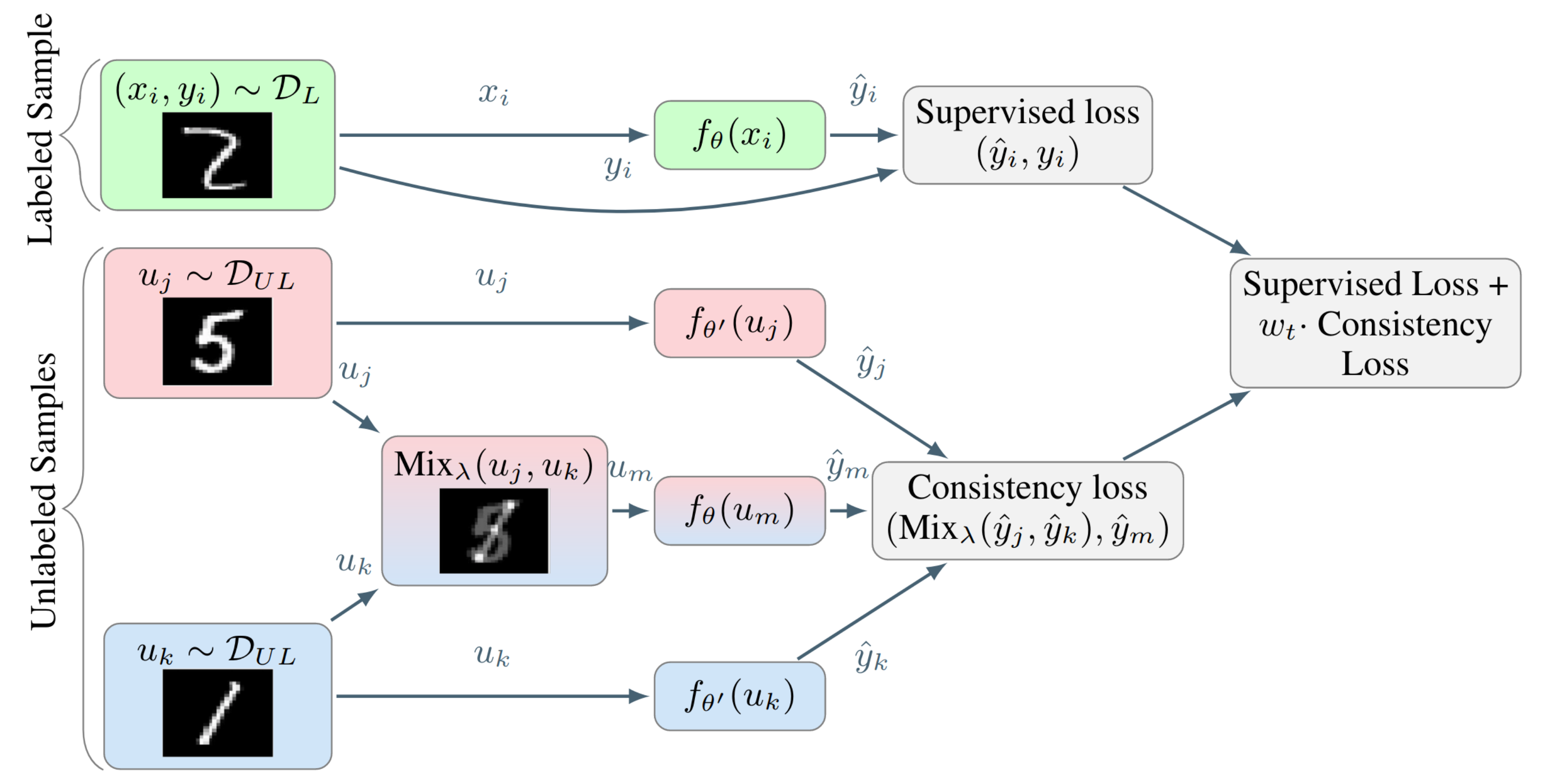

Fig. 8. ICT where a student model is trained to have consistent predictions at different interpolations of unlabeled data points, where a teacher is used to generated the targets before the mixup operation. (Image source: Verma et al)

The unsupervised objective is to have similar values between the student model’s prediction given a mixed input of two unlabeled data points and the mixed outputs of the teacher model.

\[\mathcal{L}_u = w \frac{1}{|\mathcal{D}_u|} \sum_{u_j, u_k \in \mathcal{D}_u} d_{\mathrm{MSE}}(f_{\theta}(\operatorname{Mix}_{\lambda}(u_{j}, u_{k})), \operatorname{Mix}_{\lambda}(f_{\theta^{\prime}}(u_{j}), f_{\theta^{\prime}}(u_{k}))\]

The benefit of ICT compared to random noise can be analyzed by considering the mixup operation as a perturbation applied to a given unlabeled example: \(u_{j}+\delta=\operatorname{Mix}_{\lambda}(u_{j}, u_{k})\), for a large number of classes and a with a similar distribution of examples per class, it is likely that the pair of point \(\left(u_{j}, u_{k}\right)\) lie in different clusters and belong to different classes. If one of these two data points lies in a low-density region, applying an interpolation toward \(u_{k}\) points to a low-density region, which is a good direction to move the decision boundary toward.

Unsupervised Data Augmentation

Unsupervised Data Augmentation (Xie et al.) uses advanced data augmentation methods, such as AutoAugment, RandAugment and Back Translation as perturbations for consistency training based SSL. Similar to supervised learning, advanced data augmentation methods can also provide extra advantages over simple augmentations and random noise for consistency training, given that (1) it generates realistic augmented examples, making it safe to encourage the consistency between predictions on the original and augmented examples. (2) it can generate a diverse set of examples improving the sample efficiency and (3) it is capable of providing the missing inductive biases for different tasks.

Motivated by these points, Xie et al. propose to apply the following augmentations to generate transformed versions of the unlabeled inputs:

RandAugment for Image Classification: consists of uniformly sampling from the same set of possible transformations in PIL, without requiring any labeled data to search to find a good augmentation strategy.
Back-translation for Text Classification: consists of translating an existing example in language A into another language B, and then translating it back into A to obtain an augmented example.

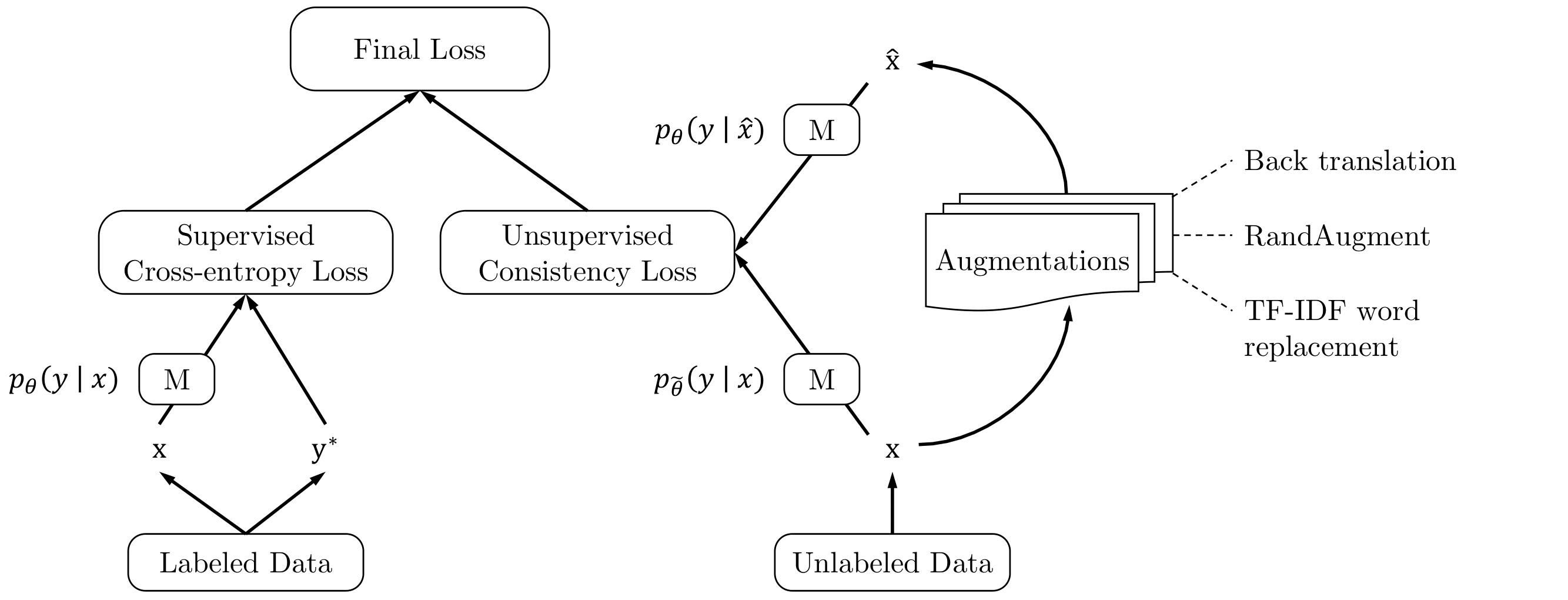
Fig. 9. The training procedure in UDA. (Image source: Qizhe Xie et al)

After defining the augmentations to be applied during training, the training procedure shown in Figure 9 is quite straight forward. The objective is to have the correct predictions over the labeled set, and consistency of predictions on the original and augmented examples from the unlabeled set.

Entropy Minimization

In the previous section, in a setting where the cluster assumption is maintained, we enforce consistency of predictions to push the decision boundary into low-density regions to avoid classifying samples from the same cluster with distinct classes, which is a violation of the cluster assumption. Another way to enforce this is to encourage the network to make confident (low-entropy) predictions on unlabeled data regardless of the predicted class, discouraging the decision boundary from passing near data points where it would otherwise be forced to produce low-confidence predictions. This is done by adding a loss term which minimizes the entropy of the prediction function \(f_\theta(x)\), e.g., for a categorical output space with \(C\) possible classes, the entropy minimization term (Grandvalet et al.) is:

\[-\sum_{k=1}^{C} f_{\theta}(x)_{k} \log f_{\theta}(x)_{k}\]

However, with high capacity models such as neural networks, the model can quickly overfit to low confident data points by simply outputting large logits, resulting in a model with very confident predictions. On its own, entropy minimization doesn’t produce competitive results compared to other SSL methods but can produce state-of-the-art results when combined with other SSL approaches.

Proxy-label Methods

Proxy label methods (Ruder et al.) are the class of SSL algorithms that produce proxy labels on unlabeled data, using the prediction function itself or some variant of it without any supervision. These proxy labels are then used as targets together with the labeled data, providing some additional training information even if the produced labels are often noisy or weak and do not reflect the ground truth, which can be divided mainly into two groups: self-training, where the model itself produces the proxy labels; and multi-view learning, where the proxy labels are produced by models trained on different views of the data.

Self-training

In self-training or bootstrapping, the small amount of labeled data \(\mathcal{D}_l\) is first used to train a prediction function \(f_{\theta}\). The trained model is then used to assign pseudo-labels to the unlabeled data points in \(\mathcal{D}_u\). Given an output \(f_{\theta}(x_u)\) for an unlabeled data point \(x_u\) in the form of a probability distribution over the classes, the pair \((x_u, \text{argmax}f_{\theta}(x_u))\) is added to the labeled set if the probability assigned to its most likely class is higher than a predetermined threshold \(\tau\). The process of training the model using the augmented labeled set and then set using it to label the remaining of \(\mathcal{D}_u\) is repeated until the model is incapable of producing confident predictions.

Pseudo-labeling can also be seen as a special case of self-training, differing only in the heuristics used to decide which proxy labeled examples to retain, such as using the relative confidence instead of the absolute confidence, where the top \(n\) unlabeled examples predicted with the highest confidence after every epoch is added to the labeled training dataset \(\mathcal{D}_l\).

The main downside of such methods is that the model is unable to correct its own mistakes and any biased and wrong classifications can be quickly amplified resulting in confident but erroneous proxy labels on the unlabeled data points.

Meta Pseudo Labels

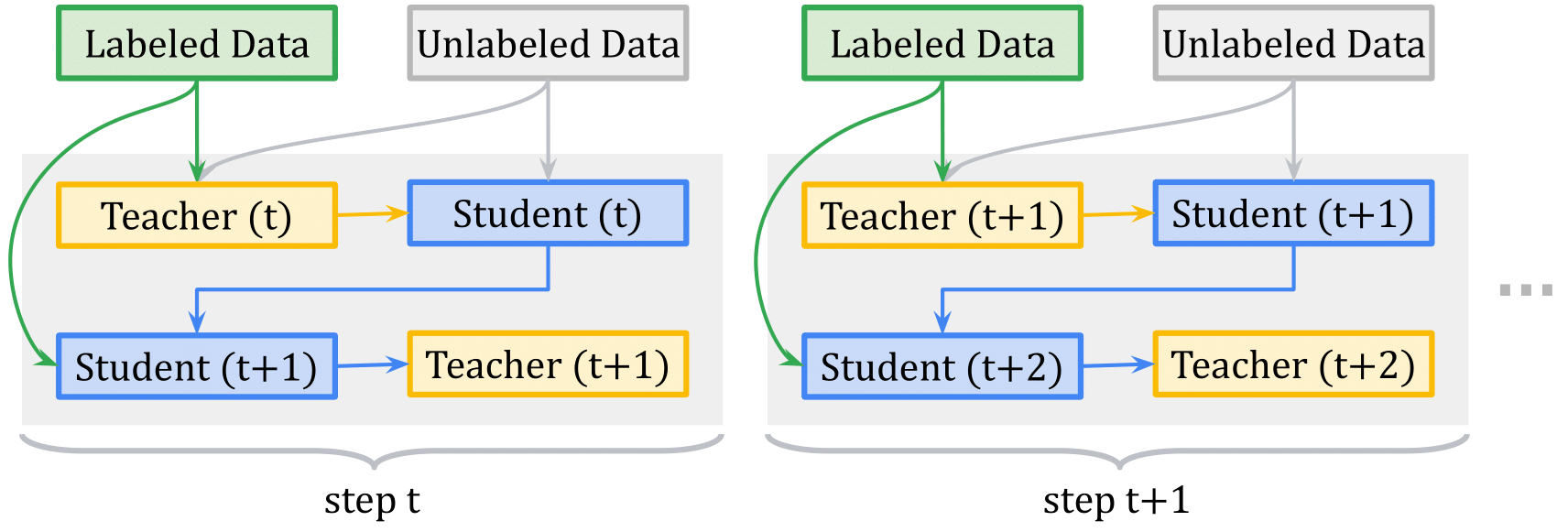
Given how important the heuristics used to generate the proxy labels, where a proper method could lead to a sizable gain. Pham et al. propose to use the student-teacher setting, where the teacher model is responsible for producing the proxy labels based on an efficient meta-learning algorithm called Meta Pseudo Labels (MPL), which encourages the teacher to adjust the target distributions of training examples in a manner that improves the learning of the student model. The teacher is updated by policy gradients computed by evaluating the student model on a held-out validation set.

A given training step of MPL consists of two phases (Figure 10):

Phase 1: The Student learns from the teacher. In this phase, given a single input example \(x_u\), the teacher \(f_{\theta^{\prime}}\) produces a target class-distribution to train the student \(f_{\theta}\), where the pair \((x_u, f_{\theta^{\prime}}(x_u))\) is shown to the student to update its parameters by back-propagating from the cross-entropy loss.
Phase 2: The Teacher learns from the Student’s Validation Loss. After the student updates its parameters in first step, its new parameter \(\theta(t+1)\) are evaluated on an example \((x_{val},y_{val})\) from the held-out validation dataset using the cross-entropy loss. Since the validation loss depends on \(\theta^{\prime}\) via the first step, this validation cross-entropy loss is also a function of the teacher’s weights \(\theta^{\prime}\). This dependency allows us to compute the gradients of the validation loss with respect to the teacher’s weights, and then update \(\theta^{\prime}\) to minimize the validation loss using policy gradients.

Fig. 10. The MPL training procedure. (Image source: Pham et al)

While the student’s performance allows the teacher to adjust and adapt to the student’s learning state, this signal alone is not sufficient to train the teacher since when the teacher has observed enough evidence to produce meaningful target distributions to teach the student, the student might have already entered a lousy region of parameters. To overcome this, the teacher is also trained using the pair of labeled data points from the held-out validation set.

Multi-view training

Multi-view training (MVL, Zhao et al.) utilizes multi-view data that are very common in real-world applications, where different views can be collected by different measuring methods (e.g., color information and texture information for images) or by creating limited views of the original data. In such a setting, MVL aims to learn a distinct prediction function \(f_{\theta_i}\) to model a given view \(v_{i}(x)\) of a data point \(x\), and jointly optimize all the functions to improve the generalization performance. Ideally, the possible views complement each other so that the produced models can collaborate in improving each other’s performance.

Co-training

Co-training (Blum et al.) requires that each data point \(x\) can be represented using two conditionally independent views \(v_1(x)\) and \(v_2(x)\), and that each view is sufficient to train a good model.

After training two prediction functions \(f_{\theta_1}\) and \(f_{\theta_2}\) on a specific view on the labeled set \(\mathcal{D}_l\). We start the proxy labeling procedure, where, at each iteration, an unlabeled data point is added to the training set of the model \(f_{\theta_i}\) if the other model \(f_{\theta_j}\) outputs a confident prediction with a probability higher than a threshold \(\tau\). This way, one of the models provides newly labeled examples where the other model is uncertain. The two views \(v_1(x)\) and \(v_2(x)\) can also be generated using consistency training methods detailed in the previous section, for example, Qiao et al. use adversarial perturbations to produce new views for deep co-training for image classification, where the models are encouraged to have the same predictions on \(\mathcal{D}_l\) but make different errors when they are exposed to adversarial attacks.

Democratic Co-training (Zhou et al.), an extension of Co-training, consists of replacing the different views of the input data with a number of models with different architectures and learning algorithms, which are first trained on the labeled examples. The trained models are then used to label a given an example \(x\) if a majority of models confidently agree on the label of an example.

Tri-Training

Tri-training (Zhou et al.) tries to reduce the bias of the predictions on unlabeled data produced with self-training by utilizing the agreement of three independently trained models instead of a single model. First, the labeled data \(\mathcal{D}_l\) is used to train three prediction functions: \(f_{\theta_1}\), \(f_{\theta_2}\) and \(f_{\theta_3}\). An unlabeled data point \(x\) is then added to the supervised training set of the function \(f_{\theta_i}\) if the other two models agree on its predicted label. The training stops if no data points are being added to any of the model’s training sets.

For a stronger heuristic when selecting the prediction to consider as proxy labels, Tri-training with disagreement (Søgaard), in addition to the only considering confident predictions with a probability higher than a threshold \(\tau\), only adds a data point \(x\) to the training set of the model \(f_{\theta_i}\) if the other two models agree, and \(f_{\theta_i}\) disagree on the predicted label. This way, the training set of a given model is only extended with data points where the model needs to be strengthened, and the easy examples that can skew the labeled data are avoided.

Using Tri-training with neural networks can be very expensive, requiring predictions for each one of the three models on all the unlabeled data. Ruder et al. propose to sample a limited number of unlabeled data points at each training epoch, the candidate pool size is increased as the training progresses and the models become more accurate. Multi-task tri-training (Ruder et al.) can also be used to reduce the time and sample complexity, where all three models share the same feature-extractor with model-specific classification layers. This way, the models are trained jointly with an additional orthogonality constraint on two of the three classification layers to be added to loss term, to avoiding learning similar models and falling back to the standard case of self-training.

Holistic Methods

An emerging line of work in SSL is a set of holistic approaches that unify the current dominant approaches in SSL in a single framework, achieving better performances.

MixMatch

Berthelot et al. propose a “holistic” approach which gracefully unifies ideas and components from the dominant paradigms for SSL, resulting in a algorithm that is greater than the sum of its parts and surpasses the performance of the traditional approaches.

MixMatch takes as input a batch from the labeled set \(\mathcal{D}_l\) containing a pair of inputs and their corresponding one-hot targets, a batch from the unlabeled set \(\mathcal{D}_u\) containing only unlabeled data, and a set of hyperparameters: sharpening softmax temperature \(T\), number of augmentations \(K\), Beta distribution parameter \(\alpha\) for MixUp. Producing a batch of augmented labeled examples and a batch of augmented unlabeled examples with their proxy labels. These augmented examples can then be used to compute the losses and train the model. Specifically, MixMatch consists of the following steps:

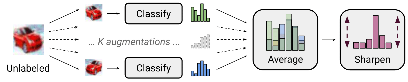
Step 1: Data Augmentation. Using a given transformation, a labeled example \(x^l\) from the labeled batch is transformed, generating its augmented versions \(\tilde{x}^l\). For an unlabeled example \(x^u\), the augmentation function is applied \(K\) times, resulting in \(K\) augmented versions of the unlabeled examples {\(\tilde{x}_1^u\), …, \(\tilde{x}_K^u\)}.
Step 2: Label Guessing. The second step consists of producing proxy labels for the unlabeled examples. First, we generate the predictions for the \(K\) augmented versions of each unlabeled example using the predictions function \(f_\theta\). The \(K\) predictions are then averaged together, obtaining a proxy or a pseudo label \(\hat{y}^u = 1/K \sum_{k=1}^{K}(\hat{y}^u_k)\) for each one of the augmentations of the unlabeled example \(x^u\): {(\(\tilde{x}_1^u, \hat{y}^u\)), …, (\(\tilde{x}_K^u, \hat{y}^u\))}.
Step 3: Sharpening. To push the model to produce confident predictions and minimize the entropy of the output distribution, the generated proxy labels \(\hat{y}^u\) in step 2 in the form of a probability distribution over \(C\) classes are sharpened by adjusting the temperature of the categorical distribution, computed as follows where \((\hat{y}^u)_k\) refers to the probability of class \(k\) out of \(C\) classes:

\[(\hat{y}^u)_k = (\hat{y}^u)_k^{\frac{1}{T}} / \sum_{k=1}^{C} (\hat{y}^u)_k^{\frac{1}{T}}\]

Step 4 MixUp. After the previous step, we created two new augmented batch, a batch \(\mathcal{L}\) of augmented labeled examples and their target, and a batch \(\mathcal{U}\) of augmented unlabeled examples and their sharpened proxy labels. Note that the size of \(\mathcal{U}\) is \(K\) times larger than the original batch given that each example \(x_u\) is replaced by its \(K\) augmented versions. In the last step, we mix these two batches. First, a new batch merging both batches is created \(\mathcal{W}=\text{Shuffle}(\text{Concat}(\mathcal{L}, \mathcal{U}))\). \(\mathcal{W}\) is then divided into two batches: \(\mathcal{W}_1\) of the same size as \(\mathcal{L}\) and \(\mathcal{W}_2\) of the same size as \(\mathcal{L}\). Using a Mixup operation that is slightly adjusted so that the mixed example is closer the labeled examples, the final step is to create new labeled and unlabeled batches by mixing the produced batches together using Mixup as follows:

\[\mathcal{L}{\prime}=\operatorname{MixUp}(\mathcal{L}, \mathcal{W}_1)\] \[\mathcal{U}{\prime}=\operatorname{MixUp}(\mathcal{U}, \mathcal{W}_2)\]

After creating two augmented batches \(\mathcal{L}{\prime}\) and \(\mathcal{U}{\prime}\) using MixMatch, we can then train the model using the standard SSL by computing the CE loss for the supervised loss, and the consistency loss for the unsupervised loss using the augmented batches as follows:

\[\mathcal{L}_s=\frac{1}{|\mathcal{L}^{\prime}|} \sum_{x_l, y \in \mathcal{L}^{\prime}} \mathrm{H}(y, f_\theta(x_l)))\] \[\mathcal{L}_u=w \frac{1}{|\mathcal{U}^{\prime}|} \sum_{x_u, \hat{y} \in \mathcal{U}^{\prime}} d_{\mathrm{MSE}}(\hat{y}, f_{\theta}(x_u))\]

ReMixMatch

Berthelot et al. propose to improve MixMatch by introducing two new techniques: distribution alignment and augmentation anchoring. Distribution alignment encourages the marginal distribution of predictions on unlabeled data to be close to the marginal distribution of ground-truth labels. Augmentation anchoring feeds multiple strongly augmented versions of the input into the model and encourages each output to be close to the prediction for a weakly-augmented version of the same input.

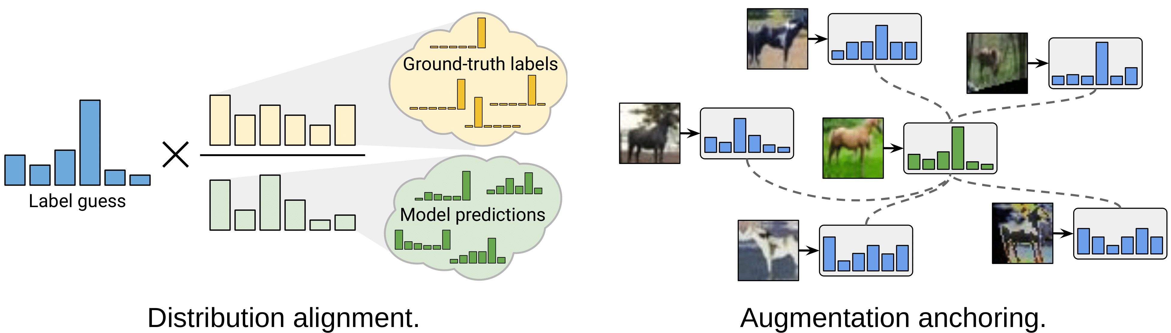
Distribution alignment: In order to force that the aggregate of predictions on unlabeled data to match the distribution of the provided labeled data. Over the course of training, a running average \(\tilde{y}\) of the model’s predictions on unlabeled data is maintained over the last 128 batches. For the marginal class distribution \(p(y)\), it is estimated based on the labeled examples seen during training. Given a prediction \(f_{\theta}(x_u)\) on the unlabeled example \(x_u\), the output probability distribution is aligned as follows: \(f_{\theta}(x_u) = \text { Normalize }(f_{\theta}(x_u) \times p(y) / \tilde{y})\).

Augmentation Anchoring: MixMatch uses a simple flip-and-crop augmentation strategy, ReMixMatch replaces the weak augmentations with strong augmentations learned using a control theory based strategy following AutoAugment. With such augmentations, the model’s prediction for a weakly augmented unlabeled image is used as the guessed label for many strongly augmented versions of the same image in a standard cross-entropy loss.

For training, MixMatch is applied to the unlabeled and labeled batches, with the application of distribution alignment and replacing the \(K\) weakly augmented example with a strongly augmented example, in addition to using the weakly augmented examples for predicting proxy labels for the unlabeled, strongly augmented examples. With two augmented batches \(\mathcal{L}^{\prime}\) and \(\mathcal{U}^{\prime}\), the supervised and unsupervised losses are computed as follows:

In addition to these losses, the authors add a self-supervised loss. First, a new unlabeled batch \(\hat{\mathcal{U}}^{\prime}\) of examples is created by rotating all of the examples with an angle \(r \sim\{0,90,180,270\}\). The rotated examples are then used to compute a self-supervised loss, where the classification layer on top of the model predicts the correct applied rotation, in addition to the cross-entropy loss over the rotated examples:

\[\mathcal{L}_{SL} = w^{\prime} \frac{1}{|\hat{\mathcal{U}}^{\prime}|} \sum_{x_u, \hat{y} \in \hat{\mathcal{U}}^{\prime}} \mathrm{H}(\hat{y}, f_\theta(x_u))) + \lambda \frac{1}{|\hat{\mathcal{U}}^{\prime}|} \sum_{x_u \in \hat{\mathcal{U}}^{\prime}} \mathrm{H}(r, f_\theta(x_u)))\]

FixMatch

Kihyuk Sohn et al. present FixMatch, a simple SSL algorithm that combines consistency regularization and pseudo-labeling. In FixMatch (Figure 13), both the supervised and unsupervised losses are computed using a cross-entropy loss. For labeled examples, the provided targets are used. For unlabeled examples \(x_u\), a weakly augmented version is first computed using a weak augmentation function \(A_w\). As in self-training, the predicted label is then considered as a proxy label if the highest class probability is greater than a threshold \(\tau\). With a proxy label for \(x_u\), \(K\) strongly augmented examples are generated using a strong augmentation function \(A_s\), we then assign to these strongly augmented versions the proxy label obtained with the weakly labeled version. With a batch of unlabeled examples of size \(\mathcal{D}_u\), the unsupervised loss can be written as follows:

\[\mathcal{L}_u = w \frac{1}{K |\mathcal{D}_u|} \sum_{x_u \in \mathcal{D}_u} \sum_{i=1}^{K} \mathbb{1}(\max (f_\theta(A_w(x_u))) \geq \tau) \mathrm{H} (f_\theta(A_w(x_u)), f_\theta(A_s(x_u)))\]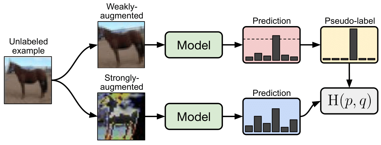

Fig. 13. FixMatch. The model prediction on a weakly augmented input is considered as target if the maximum output class probability is above threshold, this target can then be used to train the model on a strongly augmented version of the same input using standard cross-entropy loss. (Image source: Pham et al)

Augmentations. Weak augmentations consist of a standard flip-and-shift augmentation strategy. Specifically, the images are flipped horizontally with a probability of 50% on all datasets except SVHN, in addition to randomly translating images by up to 12.5% vertically and horizontally. For the strong augmentations, RandAugment and CTAugment are used where a given transformation (e.g.,, color inversion, translation, contrast adjustment, etc.) is randomly selected for each sample in a batch of training examples, where the amplitude of the transformation is a hyperparameter that is optimized during training.

Other important factors in FixMatch are the usage of adam optimizer, weight decay regularization and the learning rate schedule used, the authors propose to use a cosine learning rate decay with a decay of \(\eta \cos (\frac{7 \pi t}{16 T})\), where \(\eta\) is the initial learning rate, \(t\) is the current training step, and \(T\) is the total number of training steps.

References

^{[1] Chapelle et al. Semi-supervised learning book. IEEE Transactions on Neural Networks, 2009.

[2] Xiaojin Jerry Zhu. Semi-supervised learning literature survey. Technical report, University of Wisconsin-Madison Department of Computer Sciences, 2005.

[3] Rasmus et al. Semi-supervised learning with ladder networks. NIPS 2015.

[4] Samuli Laine, Timo Aila. Temporal Ensembling for Semi-Supervised Learning. ICLR 2017.

[5] Harri Valpola et al. From neural PCA to deep unsupervised learning. Advances in Independent Component Analysis and Learning Machines 2015.

[6] Antti Tarvainen, Harri Valpola. Mean teachers are better role models:Weight-averaged consistency targets improve semi-supervised deep learning results. NIPS 2017.

[7] Takeru Miyato et al. Virtual adversarial training: a regularization method for supervised and semi-supervised learning. Transactions on Pattern Analysis and Machine Intelligence 2018.

[8] Ian Goodfellow et al. Explaining and harnessing adversarial examples.. ICLR 2015.

[9] Sungrae Park et al. Adversarial Dropout for Supervised and Semi-Supervised Learning.. AAAI 2018.

[10] Vikas Verma et al. Interpolation Consistency Training for Semi-Supervised Learning.. IJCAI 2019.

[11] Qizhe Xie et al. Unsupervised Data Augmentation for Consistency Training.. arXiv 2019.

[12] Zhanghan Ke et al. Dual Student: Breaking the Limits of the Teacher in Semi-supervised Learning.. ICCV 2019.

[13] Sebastian Ruder et al. Strong Baselines for Neural Semi-supervised Learning under Domain Shift.. ACL 2018.

[14] Hieu Pham et al. Meta Pseudo Labels. Preprint 2020.

[15] Jing Zhao et al. Multi-view learning overview: Recent progress and new challenges. Information Fusion, 2017.

[16] Avrim Blum, Tom Michael. Combining labeled and unlabeled data with co-training., COLT 1992.
[17] Siyuan Qiao, Wei Shen, Zhishuai Zhang, Bo Wang, Alan Yuille. Deep Co-Training for Semi-Supervised Image Recognition., ECCV 2018.

[18] Yan Zhou, Sally Goldman. Democratic Co-Learning., ICTAI 2004.

[19] Zhi-Hua Zhou, Ming Li. Tri-Training: Exploiting Unlabled Data Using Three Classifiers. IEEE Trans.Data Eng 2015.

[20] Anders Søgaard. Simple Semi-Supervised Training of Part-Of-Speech Taggers. NIPS 2019.

[21] Yves Grandvalet et al. Semi-supervised learning by entropy minimization. NIPS 2005.

[22] David Berthelot et al. MixMatch: A Holistic Approach to Semi-Supervised Learning. NIPS 2019.

[23] David Berthelot et al. ReMixMatch: Semi-Supervised Learning with Distribution Matching and Augmentation Anchoring. ICLR 2020.

[24] Kihyuk Sohn et al. FixMatch: Simplifying Semi-Supervised Learning with Consistency and Confidence. Preprint 2020.}